Predicting ER status imputing missing values

Aim

The goal of this report is to predict the ER status for those patients where the ER status is unknown. To this end I used the GEO metadata downloaded in Downloading GEO data and the cluster assignments obtained in the report Identification of breast cancer subtypes and biomarkers using the Seurat workflow.

Workflow

I applied three supervised learning method (logist regression, random forest, support vector machine) and optimized their hyperparameters using a grid search using balanced accurancy as evaluation metric.
To handle missing data, I used the KNNimputer, which imputes values based on the nearest neighbors in the feature space.
For feature selection, I applied mutual_info_classif to retain the most informative features with respect to the target variable (ER status).
To address class imbalance, I set the parameter class_weight=’balanced, ensuring that the model gives appropriate attention to minority classes during training.

Conclusion

In terms of balanced accuracy, random forest slightly outperformed logistic regression and SVM.

import pandas as pd
import numpy as np
import matplotlib.pyplot as plt
from sklearn.impute import KNNImputer
from sklearn.feature_selection import SelectKBest, mutual_info_classif
from sklearn.model_selection import GridSearchCV, cross_val_score
from sklearn.linear_model import LogisticRegression
from sklearn.ensemble import RandomForestClassifier
from sklearn.svm import SVC
from sklearn.pipeline import Pipeline
from sklearn.compose import ColumnTransformer
from sklearn.preprocessing import StandardScaler, OrdinalEncoder
from IPython.display import display, HTML

Exploring dataset

Loading dataset

df = pd.read_table('data/cluster_anno_seurat.csv', sep=',')

df = df[['patient', 'age_at_diagnosis', 'tumor_size',
         'lymph_node_status','er_status', 'pgr_status', 'her2_status',
         'pam50_subtype', 'overall_survival_days', 'overall_survival_event',
         'endocrine_treated', 'chemo_treated', 'ki67_status', 'nhg',
         'seurat_clusters']]

df = df.set_index('patient')

df = df.replace({'endocrine_treated': {'no treated': 'untreated'}})
df = df.replace({'chemo_treated': {'no treated': 'untreated'}})
df = df.replace({'overall_survival_event': {'no survival': 'nosurvival'}})

df

	age_at_diagnosis	tumor_size	lymph_node_status	er_status	pgr_status	her2_status	pam50_subtype	overall_survival_days	overall_survival_event	endocrine_treated	chemo_treated	ki67_status	nhg	seurat_clusters
patient
F1	43	9.0	NodeNegative	NaN	NaN	HER2-	Basal	2367	nosurvival	untreated	treated	NaN	G3	5
F2	48	14.0	NodePositive	ER+	PgR+	HER2-	LumA	2367	nosurvival	treated	treated	NaN	G2	0
F3	69	27.0	NodePositive	ER+	PgR+	HER2-	LumB	2168	survival	treated	treated	NaN	G3	1
F4	39	51.0	NodePositive	ER+	NaN	HER2+	LumA	2416	nosurvival	treated	treated	NaN	G3	4
F5	73	60.0	NodePositive	ER+	NaN	HER2-	Normal	2389	nosurvival	treated	untreated	NaN	G2	3
...	...	...	...	...	...	...	...	...	...	...	...	...	...	...
F3269	72	13.0	NodeNegative	ER+	PgR+	HER2-	LumB	856	nosurvival	treated	treated	Ki67+	G2	7
F3270	69	30.0	NodePositive	ER+	PgR+	HER2-	LumA	861	nosurvival	treated	treated	Ki67+	G2	8
F3271	73	18.0	NodeNegative	ER+	PgR-	NaN	LumB	862	nosurvival	treated	treated	Ki67+	G3	4
F3272	67	33.0	NodePositive	ER+	PgR+	HER2-	LumA	844	nosurvival	treated	untreated	Ki67+	G2	0
F3273	60	17.0	NodePositive	ER+	PgR+	HER2-	LumA	843	nosurvival	treated	treated	Ki67+	G2	3

3273 rows × 14 columns

Missing data Distribution

features = df.columns

df_miss = df[features].isnull().sum()
df_miss = df_miss[df_miss > 0].sort_values(ascending=False)

fig, ax = plt.subplots(figsize=(10, 6))
df_miss.plot(kind='bar', ax=ax, color='skyblue', edgecolor='black')

plt.ylabel('Missing Values', fontsize=12)
plt.xticks(rotation=45, ha='right')
plt.grid(axis='y', alpha=0.3)

# Add value labels
for i, v in enumerate(df_miss.values):
  ax.text(i, v + 0.1, str(v), ha='center', va='bottom', fontweight='bold')

plt.tight_layout()
plt.show()

missperc = (len(df_miss)/len(features))*100
print(f"Tot features: {len(features)}")
print(f"Tot features with missing values: {len(df_miss)} ({missperc:0.1f}%)")
print(f"Feature with missing values: {[col for col in df_miss.index]}")
print(f"Feature without missing values: {[col for col in df.columns if col not in df_miss.index]}")

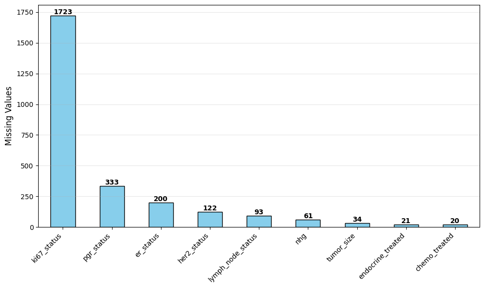
Tot features: 14
Tot features with missing values: 9 (64.3%)
Feature with missing values: ['ki67_status', 'pgr_status', 'er_status', 'her2_status', 'lymph_node_status', 'nhg', 'tumor_size', 'endocrine_treated', 'chemo_treated']
Feature without missing values: ['age_at_diagnosis', 'pam50_subtype', 'overall_survival_days', 'overall_survival_event', 'seurat_clusters']

ER status distribution

fig, ax = plt.subplots(figsize=(10, 6))
df['er_status'].value_counts(dropna=False).plot(kind='bar', ax=ax, color='skyblue', edgecolor='black')

for i, v in enumerate(df['er_status'].value_counts(dropna=False)):
  ax.text(i, v + 0.1, str(v), ha='center', va='bottom', fontweight='bold')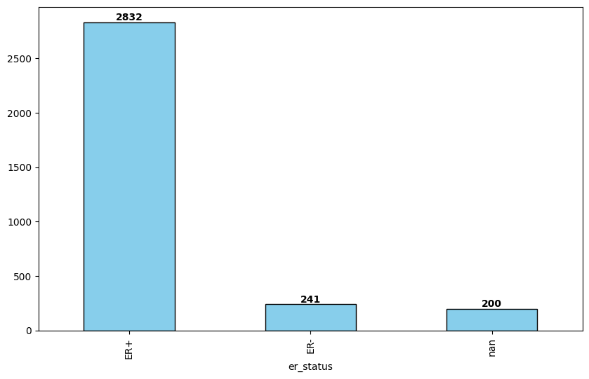

Splitting data in training and test set

y = df['er_status']
X_train, y_train = df.loc[~y.isna(),:].drop('er_status', axis=1), y[~y.isna()]
X_test, y_test = df.loc[y.isna(),:].drop('er_status', axis=1), y[y.isna()]

Imputation pipeline

def imputation_pipeline(X_train, classifier, nfeat = 5):
  # identify feature type
  categorical_features = X_train.select_dtypes(include=['object', 'category']).columns.tolist()
  numerical_features = X_train.select_dtypes(include=['int64', 'float64']).columns.tolist()

  # build imputation pipeline
  # OrdinalEncoder: designed for feature encoding, accept 2d array (X,y)
  # LabelEncoder: designed for target encoding, accept 1d array (y)
  categorical_imputer = Pipeline(steps=[
    ('encoder', OrdinalEncoder()),
    ('imputer', KNNImputer(n_neighbors=50))
  ])

  numerical_imputer = Pipeline(steps=[
    ('imputer', KNNImputer(n_neighbors=20)),
    ('scaler', StandardScaler())
  ])

  imputation = ColumnTransformer(transformers=[
    ('categorical', categorical_imputer, categorical_features),
    ('numerical', numerical_imputer, numerical_features)
  ])

  # return pipeline
  return Pipeline(steps=[
    ('imputation', imputation),
    ('feature_selection', SelectKBest(mutual_info_classif, k=nfeat)),
    ('classifier', classifier)
  ])

  ## using smote instead of class_weight='balanced'
  # from imblearn.over_sampling import SMOTE
  # from imblearn.pipeline import Pipeline as ImbPipeline
  # return ImbPipeline(steps=[
  #   ('imputation', imputation),
  #   ('smote', SMOTE(random_state=0)),  # add SMOTE after imputation
  #   ('classifier', classifier)  # remove class_weight='balanced' from classifiers
  # ])

Utility function to format results

## utils to show results
def show_results(fitted_pipeline, X_test, y_pred_proba):
  results = pd.DataFrame({
    'Patient_ID': X_test.index,
    f'Prob_{fitted_pipeline.classes_[0]}': y_pred_proba[:, 0],
    f'Prob_{fitted_pipeline.classes_[1]}': y_pred_proba[:, 1],
    'Max_Probability': np.max(y_pred_proba, axis=1),
    'Predicted_ER_Status': y_pred,
    'Confidence_Level': np.where(np.max(y_pred_proba, axis=1) > 0.8, 'High',
                        np.where(np.max(y_pred_proba, axis=1) > 0.6, 'Medium',
                      'Low'))
  }).set_index('Patient_ID')

  er_df = pd.DataFrame({
      'Label': {class_label: idx for idx, class_label in enumerate(fitted_pipeline.classes_)},
      'Count': pd.Series(y_pred).value_counts()
  }).rename_axis('ER_Status')

  confidence_df = pd.DataFrame({
      'Count': results['Confidence_Level'].value_counts(),
      'Percentage': (results['Confidence_Level'].value_counts(normalize=True) * 100).round(2)
  })

  # create side-by-side HTML
  html_str = f"""
  <div style="display: flex; gap: 50px;">
    <div>
      <h4>ER Status Distribution</h4>
      {er_df.to_html()}
    </div>          
    <div>
      <h4>Confidence Level Distribution</h4>
      {confidence_df.to_html()}
    </div>
  </div>
  """
  return results, html_str

Logistic regression

model_pipeline = imputation_pipeline(X_train, 
                                     classifier=LogisticRegression(random_state=0, max_iter=1000, class_weight='balanced'),
                                     nfeat=5)

cv_scores = cross_val_score(model_pipeline, X_train, y_train, cv=5, scoring='balanced_accuracy')
print(f"Cross-validation accuracy: {cv_scores.mean():.3f} (+/- {cv_scores.std() * 2:.3f})")

Cross-validation accuracy: 0.952 (+/- 0.062)

# Fit the final model
model_pipeline.fit(X_train, y_train)

# Make predictions on test set
y_pred = model_pipeline.predict(X_test)
y_pred_proba = model_pipeline.predict_proba(X_test)

results, html_str = show_results(model_pipeline, X_test, y_pred_proba)

display(results)
display(HTML(html_str))

	Prob_ER+	Prob_ER-	Max_Probability	Predicted_ER_Status	Confidence_Level
Patient_ID
F1	0.017625	0.982375	0.982375	ER-	High
F6	0.017625	0.982375	0.982375	ER-	High
F15	0.416440	0.583560	0.583560	ER-	Low
F16	0.017625	0.982375	0.982375	ER-	High
F27	0.026501	0.973499	0.973499	ER-	High
...	...	...	...	...	...
F2962	0.819012	0.180988	0.819012	ER+	High
F2965	0.013485	0.986515	0.986515	ER-	High
F2967	0.987457	0.012543	0.987457	ER+	High
F2976	0.982419	0.017581	0.982419	ER+	High
F3242	0.030064	0.969936	0.969936	ER-	High

200 rows × 5 columns

ER Status Distribution

	Label	Count
ER_Status
ER+	0	33
ER-	1	167

Confidence Level Distribution

	Count	Percentage
Confidence_Level
High	174	87.0
Medium	18	9.0
Low	8	4.0

Feature selection

In blue the top 5 features used in the model, in orange the discarded ones.

categorical_features = X_train.select_dtypes(include=['object', 'category']).columns.tolist()
numerical_features = X_train.select_dtypes(include=['int64', 'float64']).columns.tolist()
all_features = np.array(categorical_features + numerical_features)

feature_selector = model_pipeline.named_steps['feature_selection']
feature_index = feature_selector.get_support(indices=True)
selected_feature = all_features[feature_index]

feature_importance = pd.DataFrame({
  'Feature': all_features,
  'Score': feature_selector.scores_,
  'Selected': feature_selector.get_support()
}).sort_values('Score', ascending=False)
# display(feature_importance)

plt.figure(figsize=(10, 6))
colors = ['tab:blue' if selected else 'tab:orange' for selected in feature_importance['Selected']]
plt.barh(feature_importance['Feature'], feature_importance['Score'], color=colors)
plt.xlabel('Feature Score')
plt.gca().invert_yaxis()

# fig, ax = plt.subplots(figsize=(10, 6))
# colors = ['tab:green' if selected else 'tab:orange' for selected in feature_importance['Selected']]
# ax.barh(feature_importance['Feature'], feature_importance['Score'], color=colors)
# ax.set_xlabel('Feature Score')
# ax.invert_yaxis()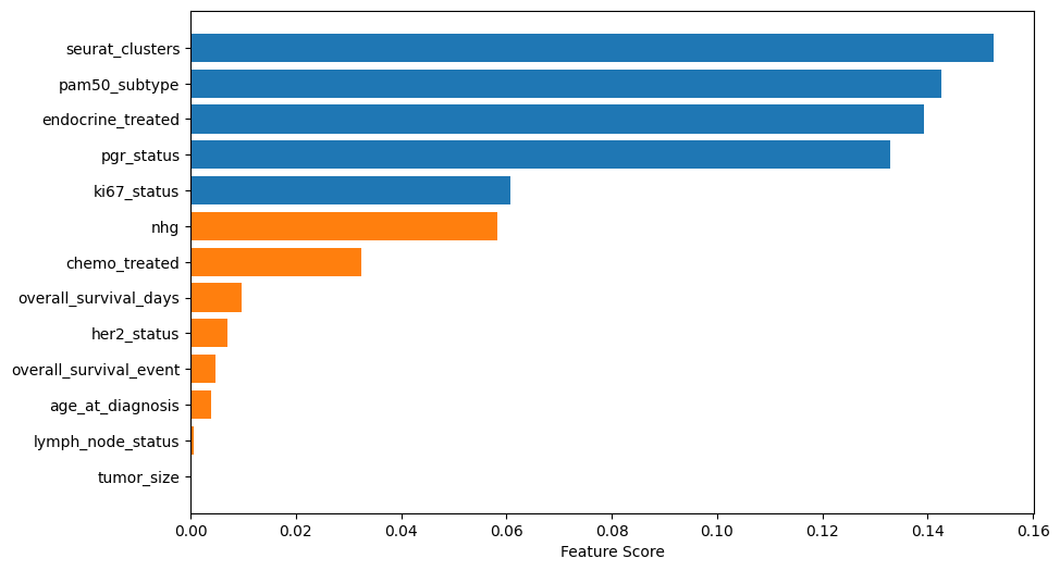

Parameter tuning

%%time

model_pipeline = imputation_pipeline(X_train,
                                     classifier= LogisticRegression(random_state=0, max_iter=1000, class_weight='balanced'),
                                     nfeat = 5)

param_grid = [
  {
    'classifier__C': [0.01, 0.1, 1, 10, 100],
    'classifier__penalty': ['l2'],
    'classifier__solver': ['lbfgs', 'newton-cholesky']
  },
  {
    'classifier__C': [0.01, 0.1, 1, 10, 100],
    'classifier__penalty': ['l1', 'l2'],
    'classifier__solver': ['liblinear', 'saga']
  },
  {
    'classifier__C': [0.01, 0.1, 1, 10, 100],
    'classifier__penalty': ['elasticnet'],
    'classifier__solver': ['saga'],  # saga is the only solver that supports elasticnet
    'classifier__l1_ratio': [0.1, 0.5, 0.7, 0.9]
  }
]

print("Starting Grid Search for Logistic Regression...")
grid_lr = GridSearchCV(
  model_pipeline, 
  param_grid, 
  cv=5, 
  scoring='balanced_accuracy', 
  n_jobs=-1, 
  verbose=1
)

# Fit the grid search
grid_lr.fit(X_train, y_train)

# Display results
print("\nBest parameters:")
print(grid_lr.best_params_)
print(f"\nAveraged cross-validation balanced accuracy score: {grid_lr.best_score_:.3f}")

Starting Grid Search for Logistic Regression...
Fitting 5 folds for each of 50 candidates, totalling 250 fits

Best parameters:
{'classifier__C': 100, 'classifier__penalty': 'l2', 'classifier__solver': 'saga'}

Averaged cross-validation balanced accuracy score: 0.955
CPU times: user 4.77 s, sys: 612 ms, total: 5.39 s
Wall time: 27.8 s

# Use the best model for predictions
best_model_lr = grid_lr.best_estimator_
y_pred = best_model_lr.predict(X_test)
y_pred_proba = best_model_lr.predict_proba(X_test)

results_lr, html_str = show_results(best_model_lr, X_test, y_pred_proba)

display(results_lr)
display(HTML(html_str))

	Prob_ER+	Prob_ER-	Max_Probability	Predicted_ER_Status	Confidence_Level
Patient_ID
F1	0.015638	0.984362	0.984362	ER-	High
F6	0.015638	0.984362	0.984362	ER-	High
F15	0.403025	0.596975	0.596975	ER-	Low
F16	0.015638	0.984362	0.984362	ER-	High
F27	0.023326	0.976674	0.976674	ER-	High
...	...	...	...	...	...
F2962	0.827821	0.172179	0.827821	ER+	High
F2965	0.011873	0.988127	0.988127	ER-	High
F2967	0.988520	0.011480	0.988520	ER+	High
F2976	0.984569	0.015431	0.984569	ER+	High
F3242	0.026950	0.973050	0.973050	ER-	High

200 rows × 5 columns

ER Status Distribution

	Label	Count
ER_Status
ER+	0	32
ER-	1	168

Confidence Level Distribution

	Count	Percentage
Confidence_Level
High	175	87.5
Medium	16	8.0
Low	9	4.5

Comparing tuned and untuned model

The tuned model slightly outperformed the untuned one.

print("Default model parameters:", model_pipeline.named_steps['classifier'].get_params())
print("Best tuned parameters:", best_model_lr.named_steps['classifier'].get_params())

# Compare probability distributions
print("\nDefault model confidence distribution:")
print(results['Confidence_Level'].value_counts())
print("\nTuned model confidence distribution:")  
print(results_lr['Confidence_Level'].value_counts())

## compare averaged cross-validated balanced accuracy 
print(f"\nAveraged cross-validated balanced accuracy (untuned model): {cv_scores.mean():.3f}")
print(f"Averaged cross-validation balanced accuracy score (tuned model): {grid_lr.best_score_:.3f}")

Default model parameters: {'C': 1.0, 'class_weight': 'balanced', 'dual': False, 'fit_intercept': True, 'intercept_scaling': 1, 'l1_ratio': None, 'max_iter': 1000, 'multi_class': 'deprecated', 'n_jobs': None, 'penalty': 'l2', 'random_state': 0, 'solver': 'lbfgs', 'tol': 0.0001, 'verbose': 0, 'warm_start': False}
Best tuned parameters: {'C': 100, 'class_weight': 'balanced', 'dual': False, 'fit_intercept': True, 'intercept_scaling': 1, 'l1_ratio': None, 'max_iter': 1000, 'multi_class': 'deprecated', 'n_jobs': None, 'penalty': 'l2', 'random_state': 0, 'solver': 'saga', 'tol': 0.0001, 'verbose': 0, 'warm_start': False}

Default model confidence distribution:
Confidence_Level
High      174
Medium     18
Low         8
Name: count, dtype: int64

Tuned model confidence distribution:
Confidence_Level
High      175
Medium     16
Low         9
Name: count, dtype: int64

Averaged cross-validated balanced accuracy (untuned model): 0.952
Averaged cross-validation balanced accuracy score (tuned model): 0.955

Random Frorest

%%time

model_pipeline = imputation_pipeline(X_train,
                                     classifier = RandomForestClassifier(random_state=0, class_weight='balanced'),
                                     nfeat=5)

param_grid = {
  'classifier__n_estimators': [50, 100, 200],
  'classifier__max_depth': [5, 10, 20, 30],
  'classifier__min_samples_split': [2, 5, 10, 20],
  'classifier__min_samples_leaf': [1, 2, 4, 8],
  'classifier__max_features': ['sqrt', 'log2']
}

# from sklearn.tree import DecisionTreeClassifier
# DecisionTreeClassifier(random_state=0)
# param_grid = {
#     'classifier__max_depth': [5, 10, 20, 30],
#     'classifier__min_samples_split': [2, 5, 10, 20],
#     'classifier__min_samples_leaf': [1, 2, 4, 8],
#     'classifier__criterion': ['gini', 'entropy'],
#     'classifier__max_features': ['sqrt', 'log2']
# }

print("Starting Grid Search for Random Forest...")
grid_rf = GridSearchCV(
  model_pipeline, 
  param_grid, 
  cv=5, 
  scoring='balanced_accuracy', 
  n_jobs=-1, 
  verbose=1
)

# Fit the grid search
grid_rf.fit(X_train, y_train)

# Display results
print("\nBest parameters:")
print(grid_rf.best_params_)
print(f"\nAveraged cross-validation balanced accuracy score: {grid_rf.best_score_:.3f}")

Starting Grid Search for Random Forest...
Fitting 5 folds for each of 384 candidates, totalling 1920 fits

Best parameters:
{'classifier__max_depth': 5, 'classifier__max_features': 'log2', 'classifier__min_samples_leaf': 8, 'classifier__min_samples_split': 10, 'classifier__n_estimators': 50}

Averaged cross-validation balanced accuracy score: 0.963
CPU times: user 19 s, sys: 954 ms, total: 19.9 s
Wall time: 3min 27s

# Use the best model for predictions
best_model_rf = grid_rf.best_estimator_
y_pred = best_model_rf.predict(X_test)
y_pred_proba = best_model_rf.predict_proba(X_test)

results_rf, html_str = show_results(best_model_rf, X_test, y_pred_proba)

display(results_rf)
display(HTML(html_str))

	Prob_ER+	Prob_ER-	Max_Probability	Predicted_ER_Status	Confidence_Level
Patient_ID
F1	0.081427	0.918573	0.918573	ER-	High
F6	0.081427	0.918573	0.918573	ER-	High
F15	0.790802	0.209198	0.790802	ER+	Medium
F16	0.081427	0.918573	0.918573	ER-	High
F27	0.105113	0.894887	0.894887	ER-	High
...	...	...	...	...	...
F2962	0.837857	0.162143	0.837857	ER+	High
F2965	0.080274	0.919726	0.919726	ER-	High
F2967	0.999465	0.000535	0.999465	ER+	High
F2976	0.999871	0.000129	0.999871	ER+	High
F3242	0.163633	0.836367	0.836367	ER-	High

200 rows × 5 columns

ER Status Distribution

	Label	Count
ER_Status
ER+	0	38
ER-	1	162

Confidence Level Distribution

	Count	Percentage
Confidence_Level
High	176	88.0
Medium	23	11.5
Low	1	0.5

SVM

%%time

model_pipeline = imputation_pipeline(X_train, 
                                     classifier= SVC(probability=True, class_weight='balanced'),
                                     nfeat=5) 


param_grid = [
  # Grid for Linear kernel
  {
    'classifier__kernel': ['linear'],
    'classifier__C': [0.01, 0.1, 1, 10, 100]
  },
  # Grid for RBF kernel
  {
    'classifier__kernel': ['rbf'],
    'classifier__C': [0.01, 0.1, 1, 10, 100],
    'classifier__gamma': [0.01, 0.1, 1, 10, 100]
  },
  # Grid for Polynomial kernel
  {
    'classifier__kernel': ['poly'],
    'classifier__C': [0.01, 0.1, 1, 10, 100],
    'classifier__degree': [2, 3, 4, 5]
  }
]

print("Starting Grid Search for SVM...")
grid_svm = GridSearchCV(
  model_pipeline, 
  param_grid, 
  cv=5, 
  scoring='balanced_accuracy', 
  n_jobs=-1, 
  verbose=1
)

# Fit the grid search
grid_svm.fit(X_train, y_train)

# Display results
print("\nBest parameters:")
print(grid_svm.best_params_)
print(f"\nAveraged cross-validation balanced accuracy score: {grid_svm.best_score_:.3f}")

Starting Grid Search for SVM...
Fitting 5 folds for each of 50 candidates, totalling 250 fits

Best parameters:
{'classifier__C': 0.1, 'classifier__gamma': 0.1, 'classifier__kernel': 'rbf'}

Averaged cross-validation balanced accuracy score: 0.961
CPU times: user 5.21 s, sys: 419 ms, total: 5.63 s
Wall time: 40.1 s

# Use the best model for predictions
best_model_svm = grid_svm.best_estimator_
y_pred = best_model_svm.predict(X_test)
y_pred_proba = best_model_svm.predict_proba(X_test)

results_svm, html_str = show_results(best_model_svm, X_test, y_pred_proba)

display(results_svm)
display(HTML(html_str))

	Prob_ER+	Prob_ER-	Max_Probability	Predicted_ER_Status	Confidence_Level
Patient_ID
F1	0.144080	0.855920	0.855920	ER-	High
F6	0.144080	0.855920	0.855920	ER-	High
F15	0.972072	0.027928	0.972072	ER+	High
F16	0.144080	0.855920	0.855920	ER-	High
F27	0.370919	0.629081	0.629081	ER-	Medium
...	...	...	...	...	...
F2962	0.979503	0.020497	0.979503	ER+	High
F2965	0.126436	0.873564	0.873564	ER-	High
F2967	0.999174	0.000826	0.999174	ER+	High
F2976	0.999446	0.000554	0.999446	ER+	High
F3242	0.380777	0.619223	0.619223	ER-	Medium

200 rows × 5 columns

ER Status Distribution

	Label	Count
ER_Status
ER+	0	27
ER-	1	173

Confidence Level Distribution

	Count	Percentage
Confidence_Level
High	147	73.5
Medium	40	20.0
Low	13	6.5

Results

Below we populate the original dataset with the predicted ER staus and the imputed values obtained by the best model (random forest) according to the averaged balanced accuracy.

pd.DataFrame({
  'Model': ['Logistic Regression',
            'Random Forest',
            'SVM'],
  'Avg_Balanced_Accuracy': [f"{grid_lr.best_score_:.3f}", 
                            f"{grid_rf.best_score_:.3f}", 
                            f"{grid_svm.best_score_:.3f}"],
}).set_index('Model').sort_values('Avg_Balanced_Accuracy', ascending=False)

	Avg_Balanced_Accuracy
Model
Random Forest	0.963
SVM	0.961
Logistic Regression	0.955

# get imputer for the best model
imputer = best_model_rf.named_steps['imputation']

# get fitted imputations
X_train_imputed = imputer.transform(X_train)
X_test_imputed = imputer.transform(X_test)

# split imputed data back into numerical and categorical parts
# nb: the slicing order is defined by ColumnTransformer in imputation_pipeline() -> categorical come before numerical features
cat_features = X_train.select_dtypes(include=['object', 'category']).columns.tolist()
num_features = X_train.select_dtypes(include=['int64', 'float64']).columns.tolist()

n_cat = len(cat_features)
n_num = len(num_features)

X_train_cat = X_train_imputed[:, :n_cat]
X_train_num = X_train_imputed[:, n_cat:n_num+n_cat]

X_test_cat = X_test_imputed[:, :n_cat]
X_test_num = X_test_imputed[:, n_cat:n_num+n_cat]

# get the ordinal encoder from the categorical transformer
categorical_transformer = imputer.named_transformers_['categorical']
ordinal_encoder = categorical_transformer.named_steps['encoder']

# inverse transform categorical features to get original labels
X_train_cat = ordinal_encoder.inverse_transform(X_train_cat)
X_test_cat = ordinal_encoder.inverse_transform(X_test_cat)

# create dataframes with original categorical values and processed numerical values
X_train_imputed = pd.DataFrame(
  np.column_stack([X_train_cat, X_train_num]),
  columns=cat_features + num_features,
  index=X_train.index
)

X_train_imputed = X_train_imputed[X_train.columns]

X_test_imputed = pd.DataFrame(
  np.column_stack([X_test_cat, X_test_num]),
  columns=cat_features + num_features,
  index=X_test.index
)

X_test_imputed = X_test_imputed[X_test.columns]

## NaN comparison
# print("Training set - original data:")
# display(X_train[X_train.isnull().any(axis=1)])

# print("\nTraining set - after imputation:")
# display(X_train_imputed[X_train.isnull().any(axis=1)])

# print("\nTest set - original data:")
# display(X_test[X_test.isnull().any(axis=1)])

# print("\nTest set - after imputation:")
# display(X_test_imputed[X_test.isnull().any(axis=1)])
## 

## complete dataset with the predicted ER status and the imputed values.
pred_er = results_svm[['Predicted_ER_Status']].rename(columns={'Predicted_ER_Status': 'er_status'})
pred_er.index.name = 'patient'
X_test_complete = pd.concat([X_test_imputed, pred_er], axis=1)

train_er = df.loc[~y.isna(), ['er_status']]
X_train_complete = pd.concat([X_train_imputed, train_er], axis=1)

display(pd.concat([X_train_complete, X_test_complete]).reindex(df.index))

## check
print("\nTot. missing values including training and test:")
print("Before imputation:", X_train.isnull().sum().sum() + X_test.isnull().sum().sum())
print("After imputation:", X_train_imputed.isnull().sum().sum() + X_test_imputed.isnull().sum().sum())

	age_at_diagnosis	tumor_size	lymph_node_status	pgr_status	her2_status	pam50_subtype	overall_survival_days	overall_survival_event	endocrine_treated	chemo_treated	ki67_status	nhg	seurat_clusters	er_status
patient
F1	-1.51916	-0.904251	NodeNegative	PgR+	HER2-	Basal	1.604754	nosurvival	untreated	treated	Ki67+	G3	0.668592	ER-
F2	-1.135531	-0.482241	NodePositive	PgR+	HER2-	LumA	1.604754	nosurvival	treated	treated	Ki67+	G2	-1.249785	ER+
F3	0.47571	0.614988	NodePositive	PgR+	HER2-	LumB	1.197026	survival	treated	treated	Ki67+	G3	-0.86611	ER+
F4	-1.826063	2.64064	NodePositive	PgR+	HER2+	LumA	1.705149	nosurvival	treated	treated	Ki67+	G3	0.284916	ER+
F5	0.782613	3.40026	NodePositive	PgR+	HER2-	Normal	1.64983	nosurvival	treated	untreated	Ki67+	G2	-0.098759	ER+
...	...	...	...	...	...	...	...	...	...	...	...	...	...	...
F3269	0.705887	-0.566643	NodeNegative	PgR+	HER2-	LumB	-1.491111	nosurvival	treated	treated	Ki67+	G2	1.435942	ER+
F3270	0.47571	0.868194	NodePositive	PgR+	HER2-	LumA	-1.480866	nosurvival	treated	treated	Ki67+	G2	1.819618	ER+
F3271	0.782613	-0.144632	NodeNegative	PgR-	HER2+	LumB	-1.478817	nosurvival	treated	treated	Ki67+	G3	0.284916	ER+
F3272	0.322258	1.121401	NodePositive	PgR+	HER2-	LumA	-1.515697	nosurvival	treated	untreated	Ki67+	G2	-1.249785	ER+
F3273	-0.214822	-0.229034	NodePositive	PgR+	HER2-	LumA	-1.517746	nosurvival	treated	treated	Ki67+	G2	-0.098759	ER+

3273 rows × 14 columns


Tot. missing values including training and test:
Before imputation: 2407
After imputation: 0