Identification of breast cancer subtypes and biomarkers using the Seurat workflow
Aims
The goal of this report is to identify breast cancer subtypes by using the Seurat workflow. In particular, we aim at validating the results obtained in the report Identification of breast cancer subtypes, where molecular subtypes were idetified by using an in-house graph-based approach.
Loading data as a Seurat object
writeMMgz <- function(x, file, threads = 10){
  mtype <- "real"
  if (is(x, "ngCMatrix")) {
    mtype <- "integer"
  }
  writeLines(
    c(
      sprintf("%%%%MatrixMarket matrix coordinate %s general", mtype),
      sprintf("%s %s %s", x@Dim[1], x@Dim[2], length(x@x))
    ),
    gzfile(file)
  )
  data.table::fwrite(
    x = summary(x),
    file = file,
    append = TRUE,
    sep = " ",
    row.names = FALSE,
    col.names = FALSE,
    nThread = threads %||% data.table::getDTthreads()
  )
}
sfile <- 'data/seurat_object.qs2'
if(!file.exists(sfile)){
dt <- fread("data/gene_expression_profile.csv.gz")
genes <- dt[[1]]
dt[, 1 := NULL] ## remove gene names column
# convert to matrix and then sparse
mx <- as.matrix(dt)
rownames(mx) <- genes
sm <- as(mx, "sparseMatrix")
writeMMgz(sm, 'data/gene_expression_matrix.mtx.gz')
write_csv(as_tibble(colnames(sm)), col_names = FALSE, file = 'data/patients.tsv.gz')
write_csv(as_tibble(rownames(sm)), col_names = FALSE, file = 'data/genes.tsv.gz')
## other way for writing the matrix on a file
# writeMM(sp, "data/expression_matrix.mtx")
# system("gzip data/gene_expression_matrix.mtx.gz")
## load sparse matrix
mx <- Seurat::ReadMtx(
mtx = 'data/gene_expression_matrix.mtx.gz',
features = 'data/genes.tsv.gz',
cells = 'data/patients.tsv.gz',
cell.column = 1, feature.column = 1
)
## load metadata
meta <- read_csv('data/metadata.csv', col_types = cols()) |>
dplyr::rename(sampleID = values, sampleName = ind) |>
dplyr::filter(sampleID %in% colnames(mx)) |>
dplyr::mutate(
er_status = factor(er_status, levels = c(0, 1), labels = c("ER-", "ER+")),
pgr_status = factor(pgr_status, levels = c(0, 1), labels = c("PgR-", "PgR+")),
her2_status = factor(her2_status, levels = c(0, 1), labels = c("HER2-", "HER2+")),
ki67_status = factor(ki67_status, levels = c(0, 1), labels = c("Ki67-", "Ki67+")),
overall_survival_event = factor(overall_survival_event, levels = c(0, 1), labels = c("no survival", "survival")),
endocrine_treated = factor(endocrine_treated, levels = c(0, 1), labels = c("no treated", "treated")),
chemo_treated = factor(chemo_treated, levels = c(0, 1), labels = c("no treated", "treated")),
lymph_node_group = factor(lymph_node_group),
lymph_node_status = factor(lymph_node_status),
pam50_subtype = factor(pam50_subtype),
nhg = factor(nhg)
) |>
tibble::column_to_rownames(var = 'sampleID')
## create seurat object
sobj <- CreateSeuratObject(mx)
sobj <- AddMetaData(sobj, metadata = meta)
## use sobj@assays$RNA$counts instead of mx to use all genes (otherwise 90 genes are filtered out)
## seurat automatically replaces '_' with '-' in gene names to avoid r syntax issues
## smx <- SetAssayData(sobj, layer = "data", new.data = mx)
## setdiff(rownames(mx), rownames(smx)) |> length() ## 90
sobj <- SetAssayData(sobj, layer = "data", new.data = sobj@assays$RNA$counts) ## already normalized data
## save and clean data
qs2::qs_save(sobj, file = 'data/seurat_object.qs2', nthreads = 10)
file.remove('data/gene_expression_matrix.mtx.gz')
file.remove('data/genes.tsv.gz')
file.remove('data/patients.tsv.gz')
}Running the Seurat workflow
sobj <- qs2::qs_read(file = 'data/seurat_object.qs2', nthreads = 10)

sobj <- Seurat::FindVariableFeatures(sobj, selection.method = "vst", nfeatures = 3000)
sobj <- Seurat::ScaleData(sobj, features = Seurat::VariableFeatures(sobj))

sobj <- Seurat::RunPCA(sobj)
sobj <- Seurat::FindNeighbors(sobj, dims = 1:25)
sobj <- Seurat::FindClusters(sobj, resolution = 1, verbose = FALSE)
sobj <- Seurat::RunUMAP(sobj, dims = 1:25)
# sobj <- RunTSNE(sobj, dims = 1:25)
Clustering evaluation
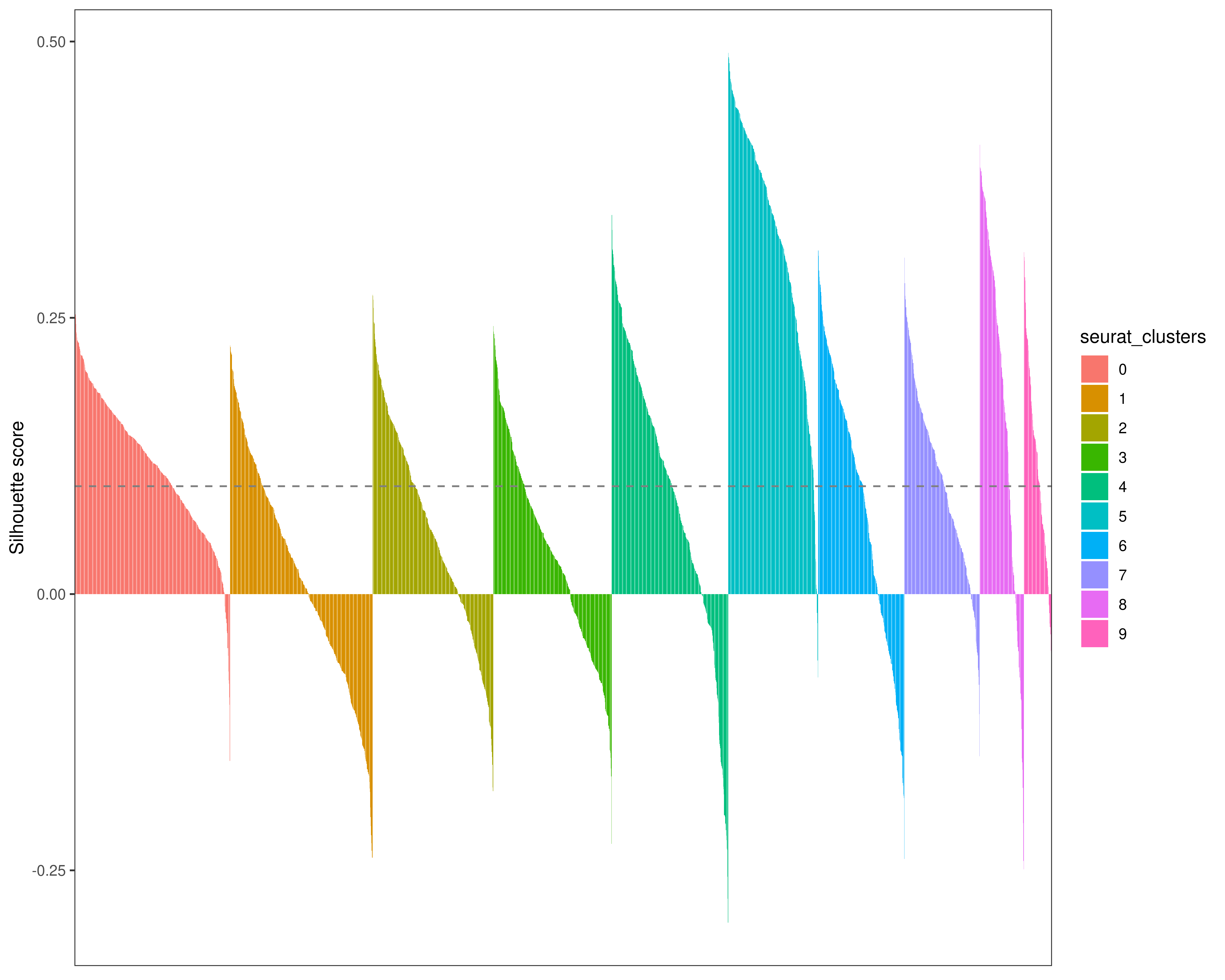
We compute a Silhouette score to evaluate how well a data point (i.e. a patient) is clustered. A positive Silhouette value means that a patient was correctly assigned to a cluster, whereas a negative value means that it is not. The larger the silhouette width, the better a patient is clustered.
## compute silhouette scores:
## https://github.com/satijalab/Integration2019/blob/master/analysis_code/integration/integration_metrics.R#L36
distance_matrix <- dist(Seurat::Embeddings(sobj[['pca']])[, 1:15])
clusters <- sobj@meta.data$seurat_clusters
silhouette <- cluster::silhouette(as.numeric(clusters), dist = distance_matrix)
sobj@meta.data$silhouette_score <- silhouette[,3]

mean_silhouette_score <- mean(sobj@meta.data$silhouette_score)

df <- sobj@meta.data |>
  dplyr::arrange(seurat_clusters, -silhouette_score) |>
dplyr::mutate(patient = factor(sampleName, levels = sampleName))ggplot(df) +
geom_col(aes(patient, silhouette_score, fill = seurat_clusters), show.legend = TRUE) +
geom_hline(yintercept = mean_silhouette_score, color = 'gray50', linetype = 'dashed') +
scale_x_discrete(name = 'Patients') +
scale_y_continuous(name = 'Silhouette score') +
theme_bw() +
theme(
axis.title.x = element_blank(),
axis.text.x = element_blank(),
axis.ticks.x = element_blank(),
panel.grid.major = element_blank(),
panel.grid.minor = element_blank()
)
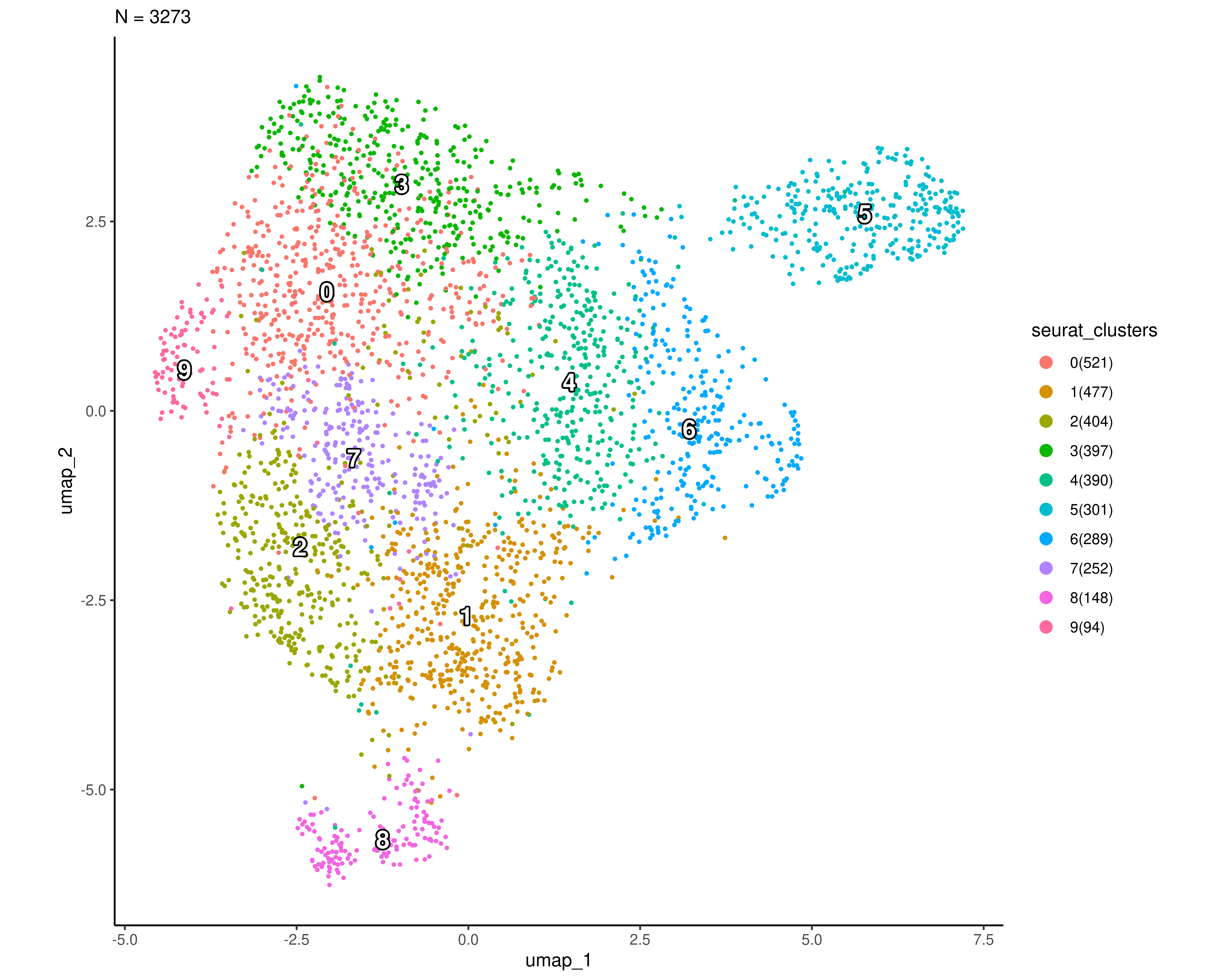
Clustering all patients
scplotter::CellDimPlot(
  sobj, group_by = "seurat_clusters", reduction = "umap",
  label = TRUE, label_insitu = TRUE, label_size = 5,
  palette = "seurat",
  theme = ggplot2::theme_classic
)
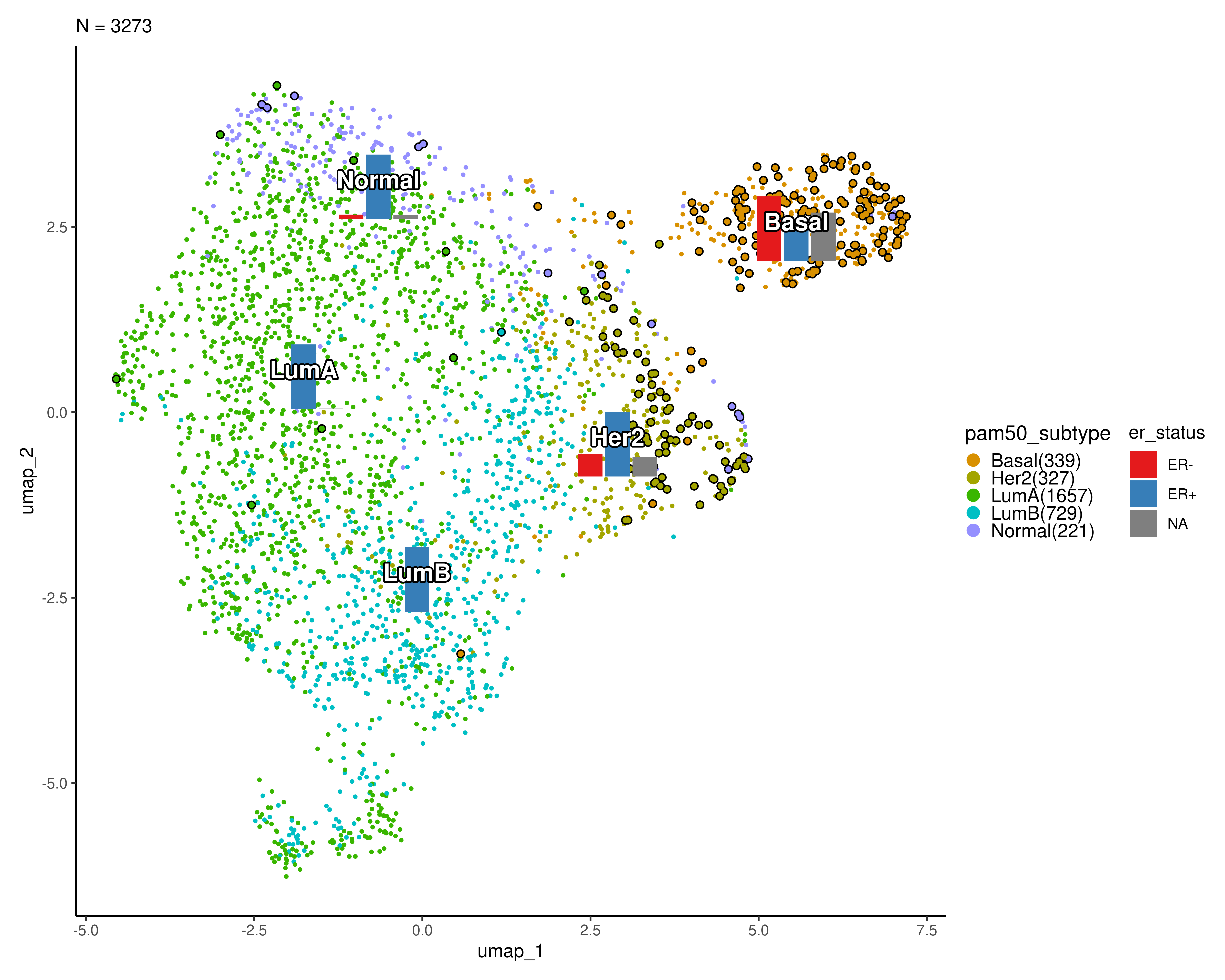
In the plot below, ER- patients are highlighted and the frequency of the ER status is shown for each cluster.
scplotter::CellDimPlot(
  sobj, group_by = "pam50_subtype", reduction = "umap",
  label = TRUE, label_insitu = TRUE, label_size = 5,
  stat_by = "er_status", stat_plot_type = "bar",
  stat_type = "count",
  stat_plot_size = 0.10,
  highlight = 'er_status == "ER-"',
  # palette = "seurat",
  palcolor = scales::hue_pal()(10)[c(2,3,4,6,8)],
  theme = ggplot2::theme_classic
  #stat_args = list(label = TRUE)
)
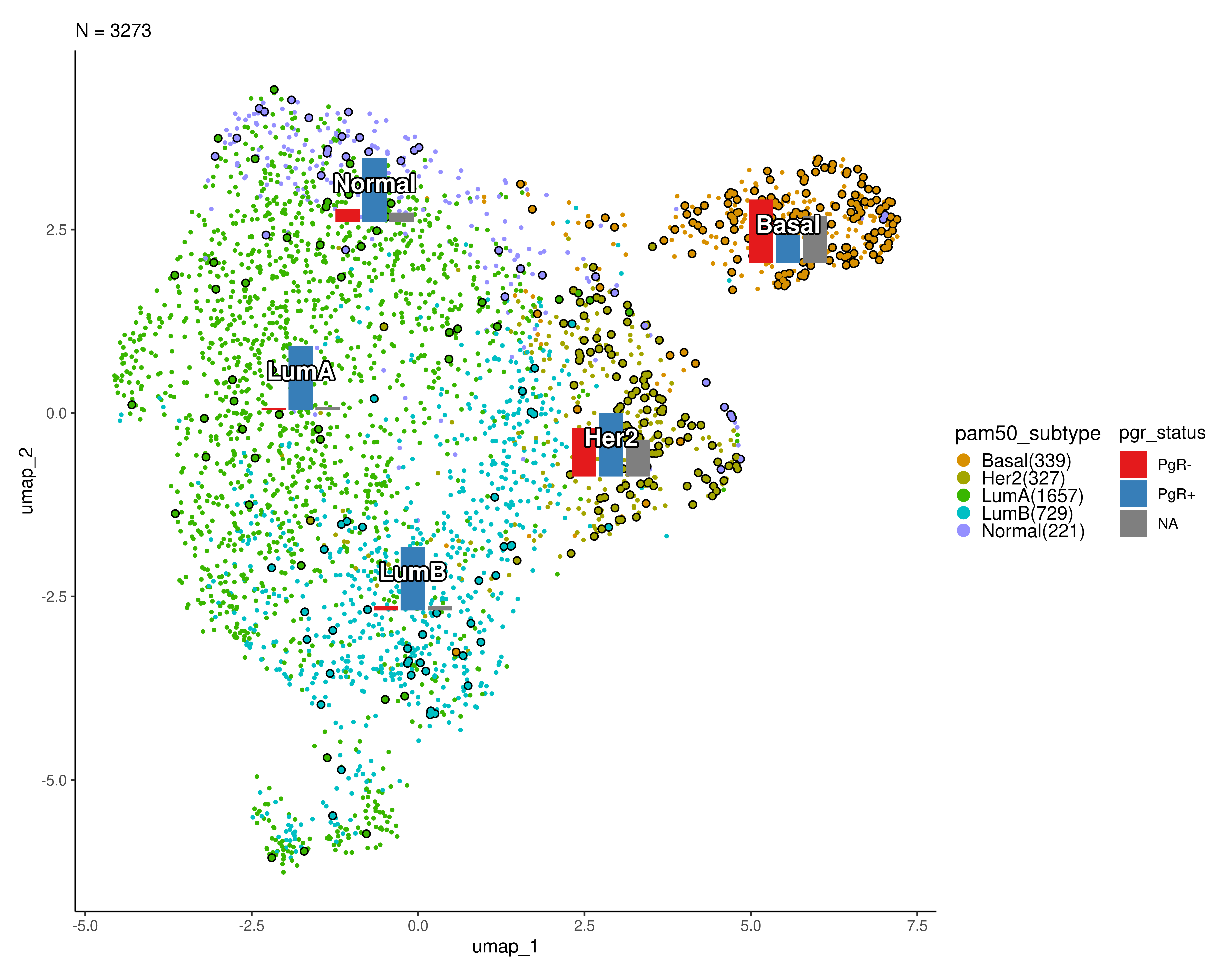
In the plot below, PgR- patients are highlighted and the frequency of the PgR status is shown for each cluster.
scplotter::CellDimPlot(
  sobj, group_by = "pam50_subtype", reduction = "umap",
  label = TRUE, label_insitu = TRUE, label_size = 5,
  stat_by = "pgr_status", stat_plot_type = "bar",
  stat_type = "count",
  stat_plot_size = 0.10,
  highlight = 'pgr_status == "PgR-"',
  # palette = "seurat",
  palcolor = scales::hue_pal()(10)[c(2,3,4,6,8)],
  theme = ggplot2::theme_classic
  #stat_args = list(label = TRUE)
)
Finding differentially expressed biomarkers
Here we aim at finding markers that define clusters via differential expression. To this end we:
- identify upregulated (positive) and downregulated (negative) markers of the Basal cluster (cluster 5) compared to all the others;
- identify up- and down-regulated markers for every cluster compared to all the others.
Moreover, we visualize the gene expression profile of some breast cancer biomarkers taken from literature (reference1 and reference2)
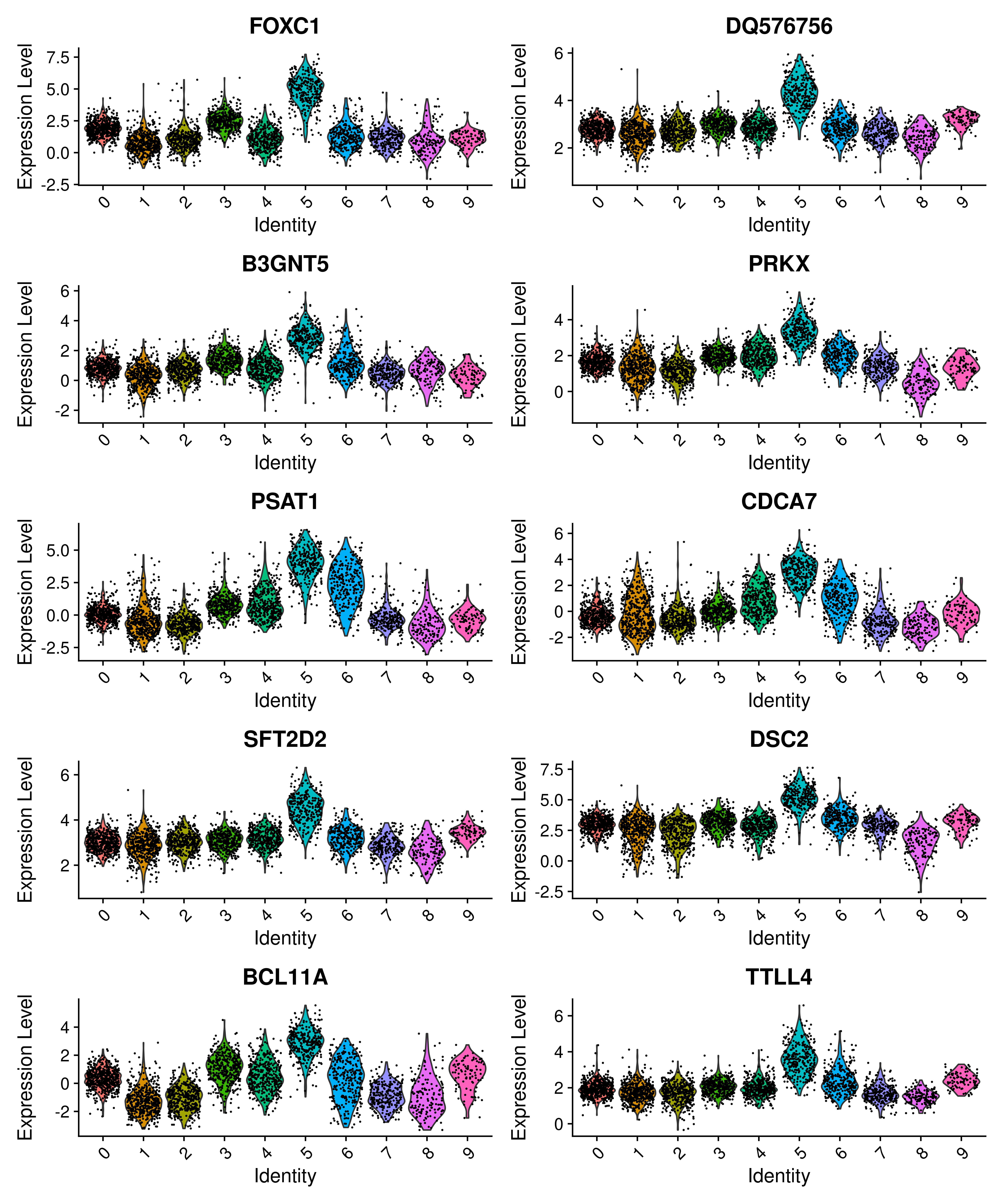
Upregulated biomarkers of the Basal cluster
basal_markers_up <- Seurat::FindMarkers(
  sobj, layer = "data",
  ident.1 = 5,
only.pos = TRUE)Seurat::FeaturePlot(
sobj, ncol = 2,
features = rownames(basal_markers_up)[1:10])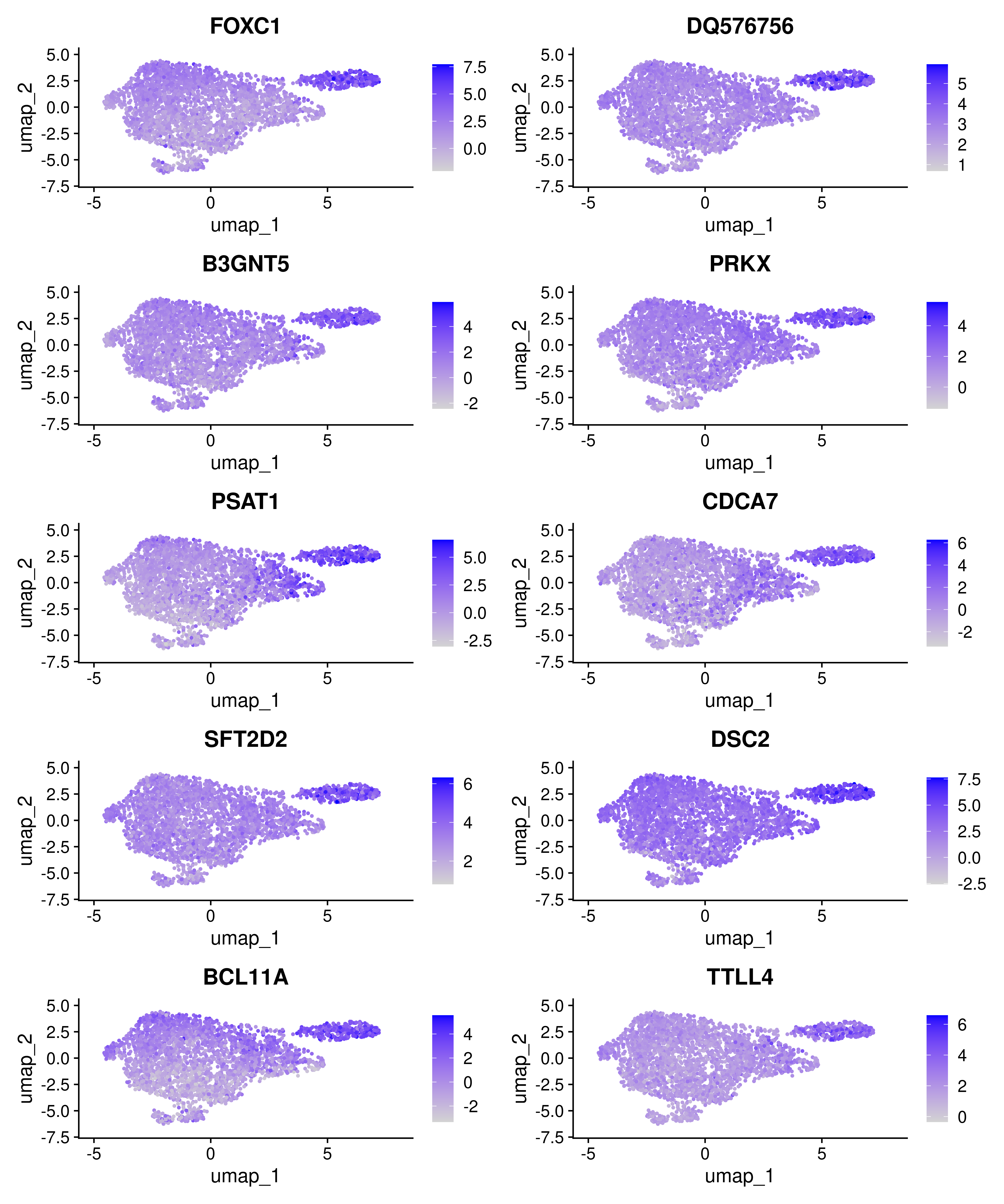
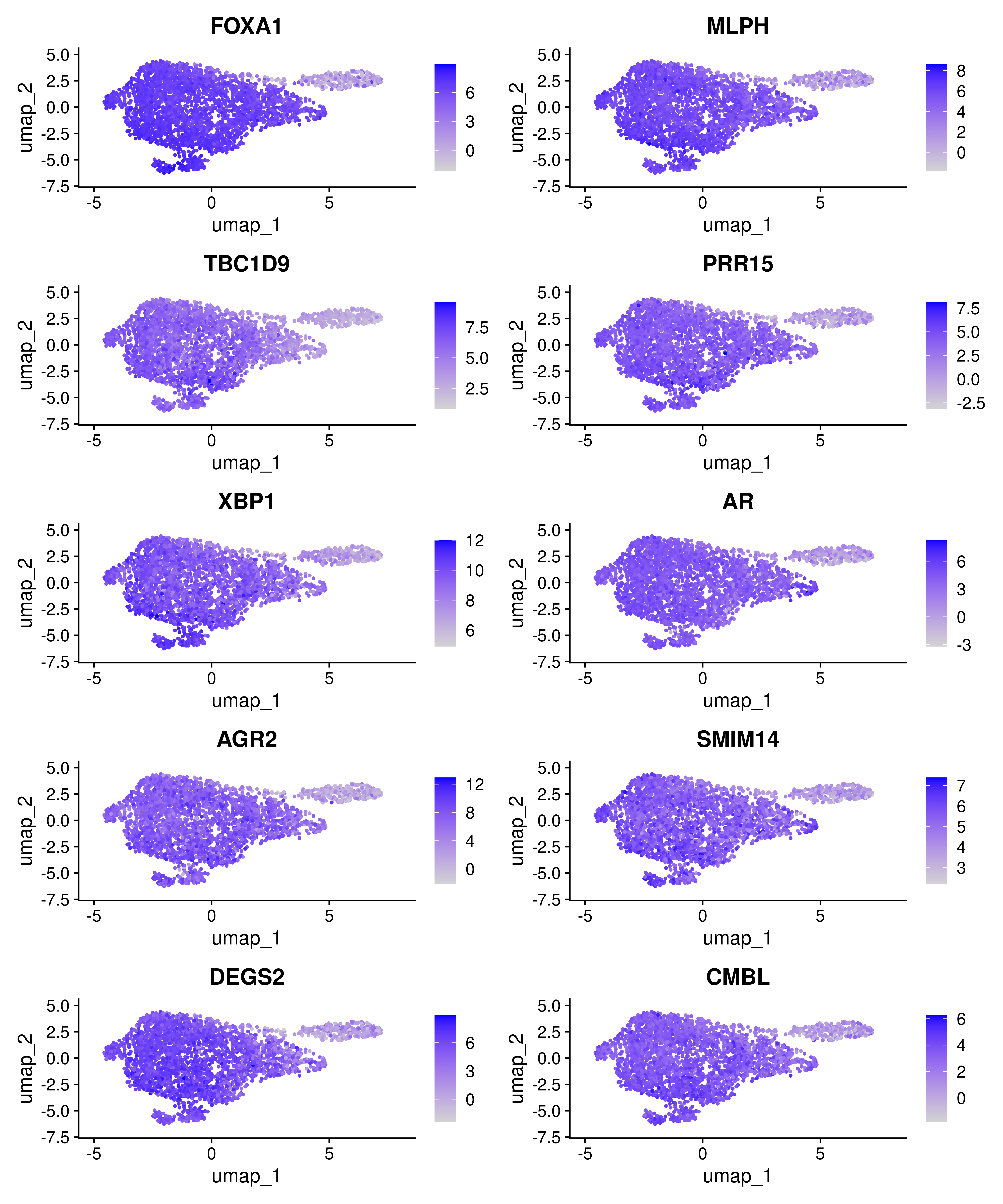
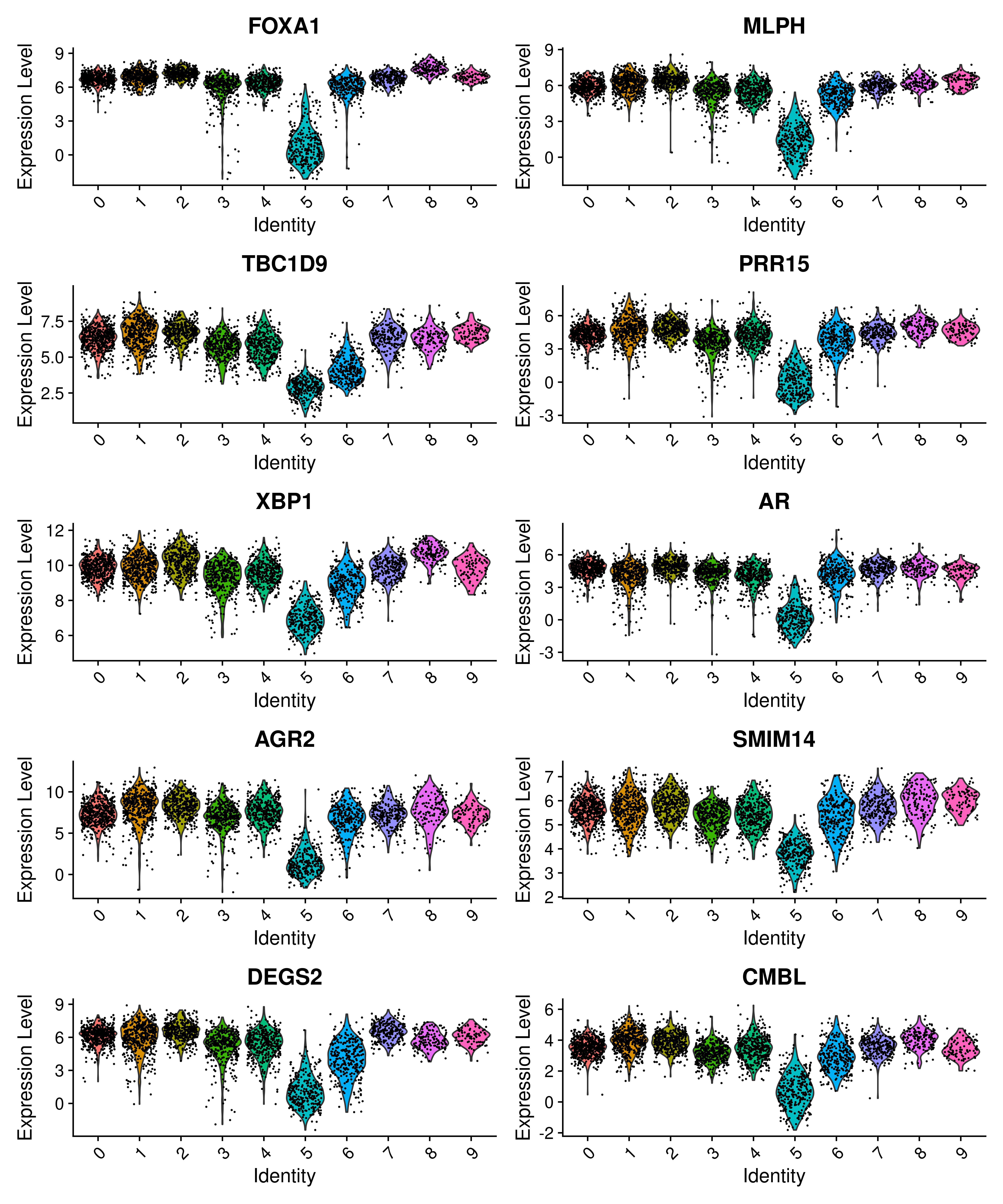
Downregulated biomarkers of the Basal cluster
basal_markers_down <- Seurat::FindMarkers(
  sobj, layer = "data",
  ident.1 = 5,
  only.pos = FALSE
)Seurat::FeaturePlot(
sobj, ncol = 2,
features = rownames(basal_markers_down)[1:10]
)
Upregulated biomarkers of all clusters
up_markers <- Seurat::FindAllMarkers(sobj, only.pos = TRUE)

top10up <- up_markers |>
  group_by(cluster) |>
  dplyr::filter(avg_log2FC > 1) |>
  dplyr::arrange(p_val_adj, avg_log2FC) |>
  slice_head(n = 10) |>
ungroup()Seurat::DoHeatmap(sobj, features = top10up$gene)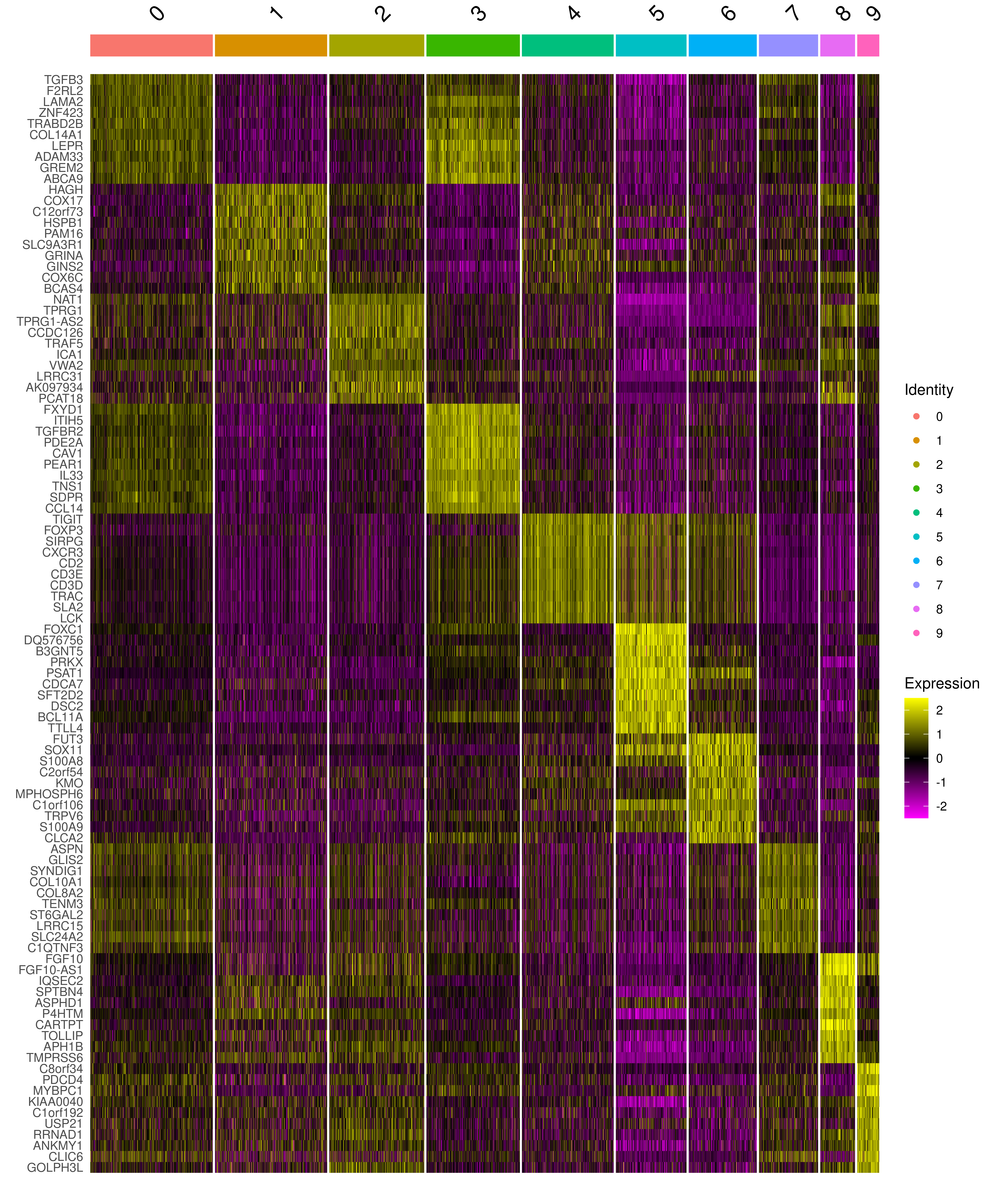
Downregulated biomarkers of all clusters
down_markers <- Seurat::FindAllMarkers(sobj, only.pos = FALSE)

top10down <- down_markers |>
  group_by(cluster) |>
  dplyr::filter(avg_log2FC < -1) |>
  dplyr::arrange(p_val_adj, avg_log2FC) |>
  slice_head(n = 10) |>
ungroup()Seurat::DoHeatmap(sobj, features = top10down$gene)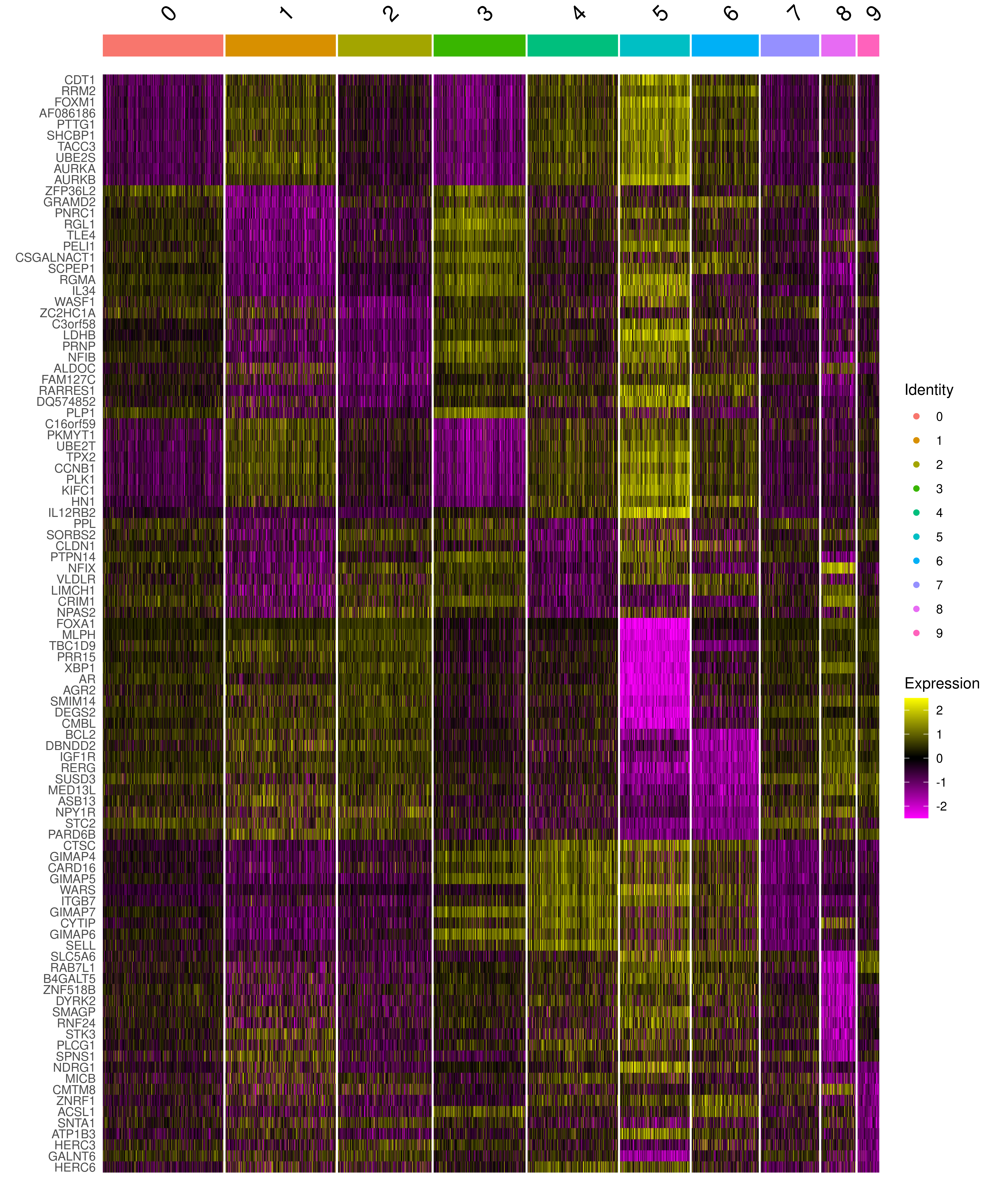
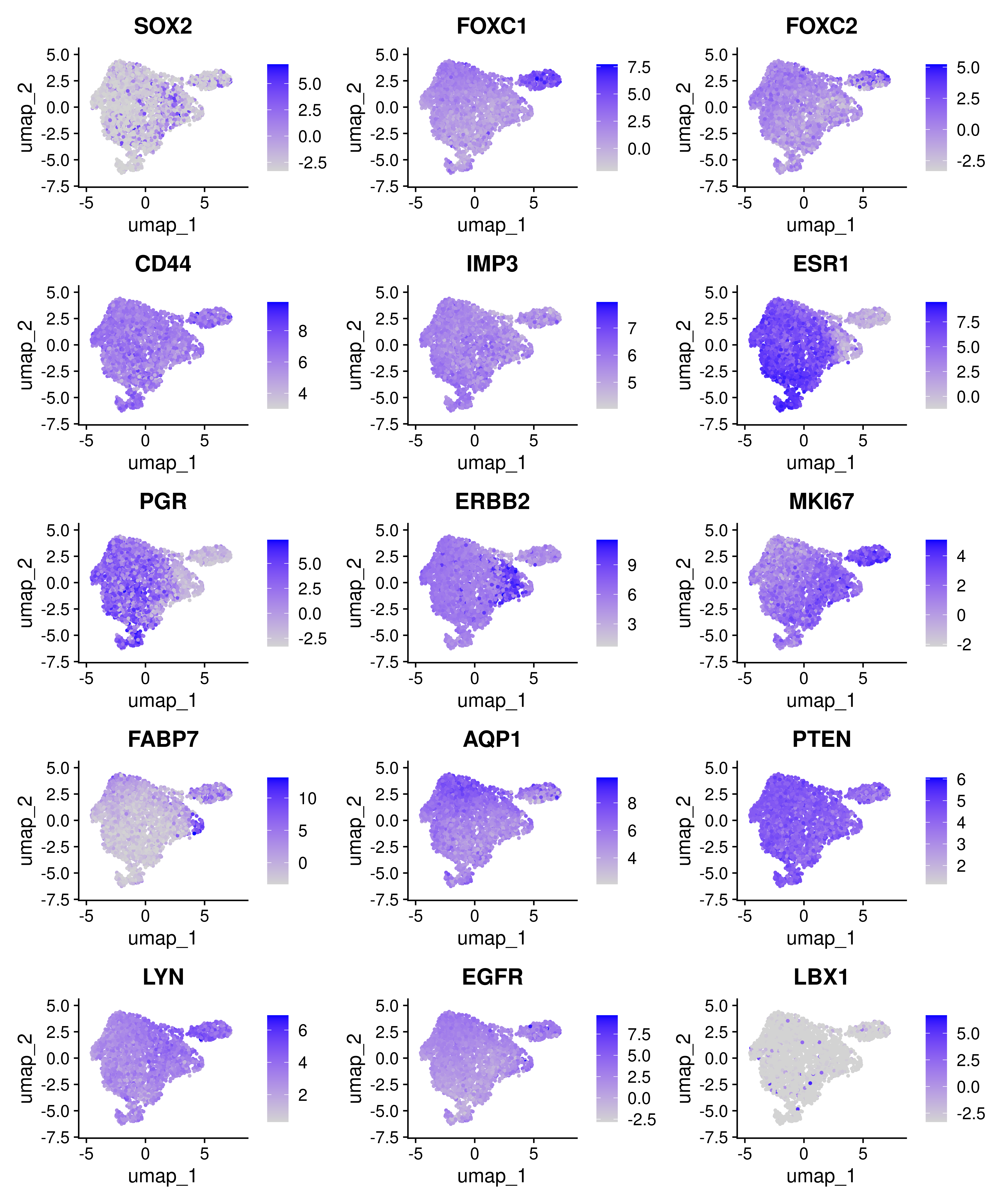
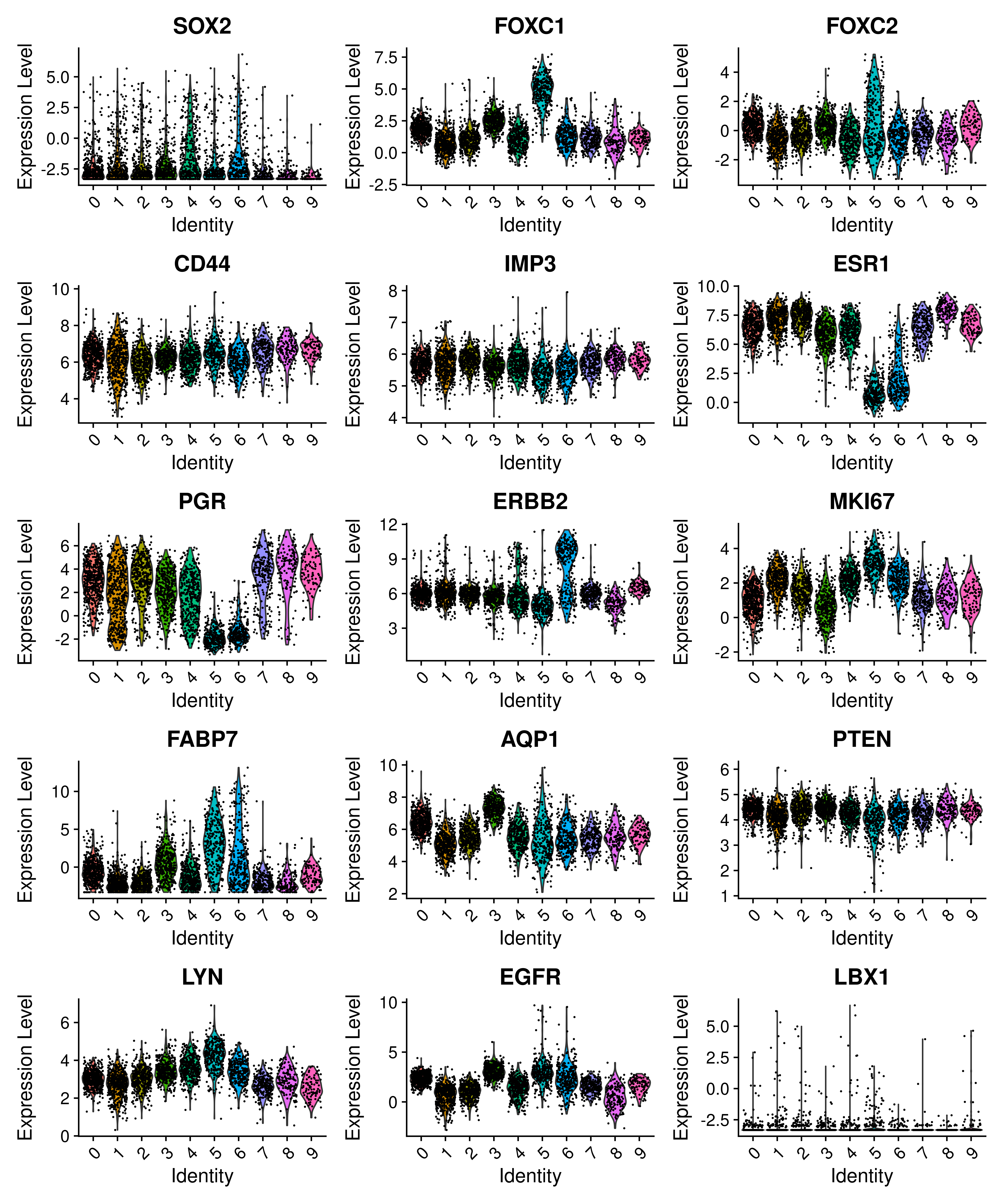
Known breast cancer biomarkers
## biomarkers for breast cancer:
##  - https://pmc.ncbi.nlm.nih.gov/articles/PMC3835118/
##  - https://pmc.ncbi.nlm.nih.gov/articles/PMC7446376/
Seurat::FeaturePlot(sobj, ncol=3,
  features = c('SOX2', 'FOXC1', 'FOXC2', 'CD44', 'IMP3', 'ESR1',
               'PGR', 'ERBB2', 'MKI67', 'FABP7', 'AQP1', 'PTEN',
               'LYN', 'EGFR', 'LBX1')
)
Check cluster assignment
To validate the two workflows, we checked that patients with the most aggressive expression profile (i.e. those in the Basal cluster) clustered in the same group. As expected, patients assigned to the Basal cluster are the same except three. The cluster assignment of the in-house workflow was downloaded from here.
## mtib downloaded from https://marconotaro.github.io/portfolio/r2_clustering.html#patient-cluster-assignment

stib <- rownames_to_column(sobj@meta.data, var = 'patient') |> as_tibble()
mtib <-  read_csv('data/cluster_anno_my_wflow.csv', col_types = cols())

mpat <- mtib |> filter(cluster==1) |> pull(sample)
spat <- stib |> filter(seurat_clusters==5) |> pull(patient)

cat('npat in mpat:', length(mpat), '\n')
npat in mpat: 304 npat in spat 301 Mode FALSE TRUE
logical 3 298 datatable <- function(tib, row2display = 10) {
if(nrow(tib) > 0){
DT::datatable(tib,
rownames = FALSE,
extensions = "Buttons",
options = list(
dom = "Bfrtip",
scrollX = TRUE,
pageLength = row2display,
buttons = list(
list(
extend = "collection",
buttons = c("csv", "excel"),
text = "Download"
)
)
),
class = "display",
style = "bootstrap"
)
}else{
print("No results")
}
}
formatter <- function(tib, cols_to_format = "all", digits = 3){
selector <- if(length(cols_to_format) == 1 && cols_to_format == "all"){
where(is.numeric)
} else {
all_of(cols_to_format)
}
tib |>
mutate(across({{ selector }},
~format(., scientific = TRUE, digits = digits)))
}
# write_csv(stib, file = 'data/cluster_anno_seurat.csv')
stib |>
formatter(cols_to_format = c("nCount_RNA", "silhouette_score")) |>
datatable()Conclusion
As expected, the clustering results obtained with the Seurat workflow are consistent wih those shown in the report Identification of breast cancer subtypes.
Next step
Cluster assignment can be used to train supervised machine learning models to predict the ER status for those patients where the ER status is unknown.